WPF Menu “Tab” Style

Background

Earlier this month, I decided to investigate how I could style the menus in my tools to look like tabs, similar to how they are styled in Visual Studio.

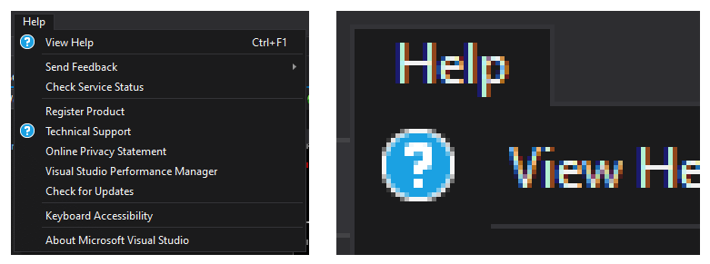
As an example, here is the Help menu in Visual Studio 2019. Notice how there is no edge under the “Help” text.

Visual Studio - Help Menu

While I’m sure there are multiple ways of achieving this style, I like the approach described in Menus with Style. However, the post is a guide for how to create this visual style via Blend. I don’t use Blend to edit my styles, so found the guide to be a bit difficult to follow. As such, I figured that it might be a good idea to write up an article that walks through the same design purely in XAML.

Overview

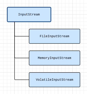
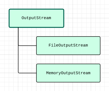
There are two components to the ControlTemplate: the Menu and the Popup.

The Menu component is covered by a single part:

  • MenuBackground (shown in green)

The Popup is split into two pieces:

  • SubmenuBorder_Left (shown in blue)
  • SubmenuBorder_Right (shown in red)

Menu - Component Diagram

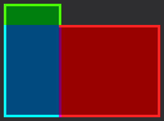
For each part, I’ve highlighted the borders that are required to make up the final style.

Also, you have probably noticed the small strip of purple. This represents an overlap of the blue and red parts, which we will discuss that shortly.

In XAML, we will use the Border element for each of these pieces, since it provides a border edge and background.

One final point before we begin. In this article, I’m using a border edge size of 1 to match the Visual Studio style shown above. However, this approach will work with any edge size.

Menu

There’s nothing too special about the MenuBackground portion so I won’t spend much time here.

From the diagram, we can see that we need border edges along the Left, Top, and Right.

<Border
   x:Name="MenuBackground"
   ...
   BorderThickness="1,1,1,0"
   />

Popup

The key thing to recognize in the diagram above is that the SubmenuBorder_Left must match the width of the MenuBackground. We can do this by binding the Width property to the MenuBackground‘s ActualWidth:

<Border
   x:Name="SubmenuBorder_Left"
   Width="{Binding ElementName=MenuBackground, Path=ActualWidth}"
   ...
   />

With this in place, we can now assemble the Popup background and border. We use a DockPanel to layout the pair of Border elements. The SubmenuBorder_Left is docked on the Left, while the SubmenuBorder_Right fills the rest of the DockPanel area.

Using the diagram above as a guide, the BorderThickness for each part is straightforward:

SubmenuBorder_Left  :   Left,    0,      0,  Bottom
SubmenuBorder_Right :      0,  Top,  Right,  Bottom

Again, I’m using a border edge size of 1 (as you’ll see the in the XAML below).

<DockPanel LastChildFill="True">
   <Border
      x:Name="SubmenuBorder_Left"
      DockPanel.Dock="Left"
      Background="{StaticResource SubmenuBackgroundBrush}"
      BorderBrush="{StaticResource SubmenuBorderBrush}"
      BorderThickness="1,0,0,1"
      Width="{Binding ElementName=MenuBackground, Path=ActualWidth}"
      />
   <Border
      x:Name="SubmenuBorder_Right"
      Margin="-1,0,0,0"
      Background="{StaticResource SubmenuBackgroundBrush}"
      BorderBrush="{StaticResource SubmenuBorderBrush}"
      BorderThickness="0,1,1,1"
   />
</DockPanel>

Overlap

As promised, let’s discuss the overlap.

The overlap is produced by the negative margin of SubmenuBorder_Right: -1, 0, 0, 0.

The purpose of this overlap is to produce the corner between the top edge of the popup (in red) and the right edge of the menu item (in green). Without it, there would be a notch in the border edge (as demonstrated below).

Menu - Component Diagram - Overlap Comparison

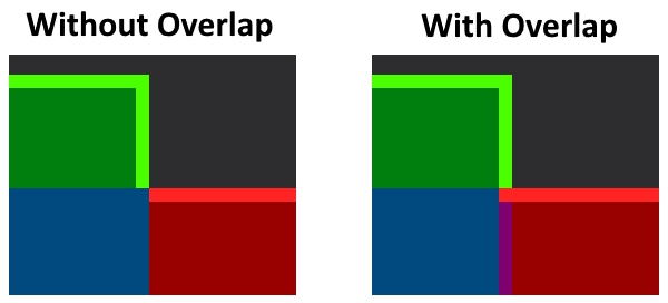
To be clear, the overlap value should match the border edge size (as mentioned earlier, the border edge size is 1).

Final Result

Putting it all together, here are the relevant parts to the ControlTemplate XAML:

<ControlTemplate
   x:Key="{ComponentResourceKey
      ResourceId=TopLevelHeaderTemplateKey,
      TypeInTargetAssembly={x:Type MenuItem}}"
   TargetType="{x:Type MenuItem}"
   >
   <Grid SnapsToDevicePixels="True">

      <!-- Background and Border -->
      <Border
         x:Name="MenuBackground"
         Margin="1"
         Background="{TemplateBinding Background}"
         BorderBrush="Transparent"
         BorderThickness="1,1,1,0"
         />

      <!-- Content -->
      <!-- ... -->


      <!-- Popup -->
      <Popup
         x:Name="PART_Popup"
         AllowsTransparency="True"
         Focusable="False"
         IsOpen="{Binding IsSubmenuOpen, RelativeSource={RelativeSource TemplatedParent}}"
         Placement="Bottom"
         HorizontalOffset="1"
         VerticalOffset="-1"
         >
         <Grid>

            <!-- Submenu Background and Border -->
            <DockPanel LastChildFill="True">
               <Border
                  x:Name="SubmenuBorder_Left"
                  DockPanel.Dock="Left"
                  Background="{StaticResource SubmenuBackgroundBrush}"
                  BorderBrush="{StaticResource SubmenuBorderBrush}"
                  BorderThickness="1,0,0,1"
                  Width="{Binding ElementName=MenuBackground, Path=ActualWidth}"
                  />
               <Border
                  x:Name="SubmenuBorder_Right"
                  Margin="-1,0,0,0"
                  Background="{StaticResource SubmenuBackgroundBrush}"
                  BorderBrush="{StaticResource SubmenuBorderBrush}"
                  BorderThickness="0,1,1,1"
                  />
            </DockPanel>

            <!-- Content -->
            <!-- ... -->

         </Grid>
      </Popup>
   </Grid>

   <ControlTemplate.Triggers>
      <Trigger Property="IsSubmenuOpen" Value="True">
         <Setter TargetName="MenuBackground" Property="Background" Value="{StaticResource SubmenuBackgroundBrush}" />
         <Setter TargetName="MenuBackground" Property="BorderBrush" Value="{StaticResource SubmenuBorderBrush}" />
      </Trigger>
   </ControlTemplate.Triggers>
</ControlTemplate>

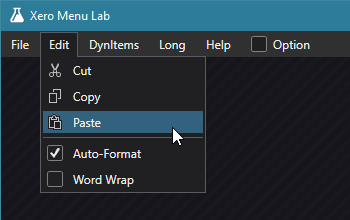
Here is a screenshot of this style used my test application.

Xero - Menu Lab: Edit Menu

Nullptr

This last week, I spent a couple days converting all of the uses of NULL in Sauce to nullptr. As such, I wanted to take this opportunity to jot down some notes on what the differences are and why I believe that it is worth your time to convert your own code to use nullptr if you haven’t already.

NULL

Similar to many other C++ code bases, Sauce used the following code to define NULL:

#if !defined(NULL)
   #define NULL 0
#endif

While it is true that many commercial software packages and games have shipped with this definition of NULL, it is still problematic.

The reason why is that NULL is simply an integer, not an actual null pointer. The danger stems from the fact that other constructs can be implicitly converted to and from integers. This means that using NULL can hide bugs.

In fact, I’ll be the first to admit that during the transition to nullptr, I found a few of these types of conversion errors in Sauce. Sure, the code still compiled and ran — but it was a bit disheartening to find them nonetheless.

Nullptr

Unlike NULL, nullptr is a keyword (available starting in C++11). It is defined to be implicitly converted to any pointer type, but cannot be implicitly converted to an integer. This allows the compiler to recognize the sort of type mismatches we hope that it would.

Let’s walk through an example to see the difference.

An Example

The problem we will explore in this example is the fact that booleans can be compared with NULL without a compiler warning. This is because the C++ standard declares that there is an implicit conversion from bool to int.

// signature:
Result* DoSomething();
 
// client code:
if (DoSomething() == NULL)
   printf("NULL\n");
else
   printf("NOT NULL\n");

Although this example is a bit contrived, the danger it exemplifies is real.

What happens if we change the return type of DoSomething() from Result* to bool? A change like this is certainly not unheard of — instead of using a full object, maybe we feel like we can reduce the result to a simple boolean.

// signature:
bool DoSomething();
 
// client code:
if (DoSomething() == NULL)
   printf("NULL\n");
else
   printf("NOT NULL\n");

The code still compiles — no additional warnings (even on Warning level 4!). That seems wrong… checking if a boolean is equal to null pointer is nonsensical and the compiler should bark when it comes across code like this, right?

Unfortunately, the compiler can’t detect the issue because we are using a #define as a stand-in for a null pointer. Remember, it’s not really a null pointer, it’s just the same value that a null pointer evaluates to: 0. Therefore, we shouldn’t be surprised when corner cases like this result in unexpected behavior.

So what happens if we replace NULL with the nullptr keyword?

// signature:
bool DoSomething();
 
// client code:
if (DoSomething() == nullptr)
   printf("NULL\n");
else
   printf("NOT NULL\n");

Now the compiler will generate an error stating that there is no conversion from 'nullptr' to 'int'. This is much better. We know that there is a type mismatch in the comparison, and we can repair the issue.

Final Thoughts

Simply put, the nullptr keyword is a true null pointer, while NULL is not.

When I was first deciding whether I was going to undertake the conversion task, I felt a bit overwhelmed at the number of changes that I would have to make (at the time there were over 5000 instances of NULL in Sauce). However, as I mentioned earlier, had I not made the transition to nullptr, those silent implicit conversion bugs would surely still be there. As such, I feel that Sauce is far better off with nullptr.

Scoped Enums

For the most part, I really like the C++ language. That said, I also have a small list of things that I wish had been done differently. For years, enumerations have been at the top of that list. Enums have a couple of distinct problems that make them troublesome, and while there are techniques to mitigate some of their issues, they still remain fundamentally flawed.

Thankfully, C++11 added scoped enums (or “strongly-typed” enums), which address these problems head-on. In my opinion, the best part about scoped enums is that the new syntax is intuitive and feels natural to the C++ language.

In an effort to build a case for why scoped enums are superior, we will first discuss the aforementioned deficiencies of their unscoped counterparts. Throughout this discussion we will also outline how we addressed some of these concerns in Sauce. Afterward, we will explore scoped enums and the task of transitioning Sauce to use them.

Terminology

Before we begin, let’s briefly establish some terminology. An unscoped enum has the following form:

enum IDENTIFIER
{
   ENUMERATOR,
   ENUMERATOR,
   ENUMERATOR,
};

The identifier is also referred to as the “type” of the enum. The list inside the enum is composed of enumerators. Each enumerator has an integral value.

Problem 1: Enumerators are treated as integers inside the parent scope.

Aliased Values

Consider the case where you have two enums inside the same parent scope. Unfortunately, there is no reinforcement by the compiler to say that a given enumerator is associated with one enum over the other. This can cause a couple issues. Here’s an example:

namespace Example1
{
   enum Shape
   {
      eSphere,
      eBox,
      eCone,
   };
 
   enum Material
   {
      eColor,
      eTexture,
   };
}

Now let’s see what happens when we try to use these enums in some client code:

const Example1::Shape shape = Example1::eSphere;
if (shape == Example1::eSphere)
   printf("SPHERE\n");
if (shape == Example1::eBox)
   printf("BOX\n");
if (shape == Example1::eCone)
   printf("CONE\n");
 
if (shape == Example1::eColor)
   printf("COLOR\n");
if (shape == Example1::eTexture)
   printf("TEXTURE\n");

The code above prints out both “SPHERE” and “COLOR”. This is because unscoped enum enumerators are implicitly converted to integers and the value of shape is 0, which matches both eSphere and eColor.

Sadly, the only workable solution is to manually assign a value to each of the enumerators that is unique within the parent scope. This is far from ideal due to the added maintenance cost.

Enumerator Name Clashes

Additionally, there is a second issue that arises from the fact that enums are swallowed into their parent scope: enumerator name clashes. For instance, consider modifying the previous case to add an “invalid” enumerator to each enum. While this makes sense conceptually, the following code will not compile:

namespace Example2A
{
   enum Shape
   {
      eInvalid,
      eSphere,
      eBox,
      eCone,
   };
 
   enum Material
   {
      eInvalid,
      eColor,
      eTexture,
   };
}

Although enumerator name clashes are not too common, it is generally bad practice to establish coding conventions that depend on the rarity of such situations.

Consequently, this usually forces you to mangle the enumerator names to include the enum type. Modifying the previous example might look something like this:

namespace Example2B
{
   enum Shape
   {
      eShape_Invalid,
      eShape_Sphere,
      eShape_Box,
      eShape_Cone,
   };
 
   enum Material
   {
      eMaterial_Invalid,
      eMaterial_Color,
      eMaterial_Texture,
   };
}

This version of the code will compile, but now the enumerator names look a little weird. Also, it is important to point out that we are now repeating ourselves: the enum identifier and each of the enumerators.

Another way to solve the name clash issue is to wrap the enum with an additional scoping object: namespace, class, or struct. Employing this method will allow us to keep our original enumerator names, which I like. However, it actually introduces a new problem: now we need two names… one for the scope and one for the enum itself.

Admittedly, there are a few different ways to handle this, but for the sake of the example let’s keep things simple:

namespace Example2C
{
   namespace Shape
   {
      enum Enum
      {
         eInvalid,
         eSphere,
         eBox,
         eCone,
      };
   };
 
   namespace Material
   {
      enum Enum
      {
         eInvalid,
         eColor,
         eTexture,
      };
   };
}

While the extra nesting does make the declaration a bit ugly, it solves the enumerator name clash problem. Furthermore, it also forces client code to prefix enumerators with their associated scoping object, which I personally consider a big win.

// in some Example2C function...
 
const Shape::Enum shape = GetShape();
if (shape == Shape::eInvalid)
   printf("Shape::Invalid\n");
if (shape == Shape::eSphere)
   printf("Shape::Sphere\n");
if (shape == Shape::eBox)
   printf("Shape::Box\n");
if (shape == Shape::eCone)
   printf("Shape::Cone\n");
 
const Material::Enum material = GetMaterial();
if (material == Material::eInvalid)
   printf("Material::Invalid\n");
if (material == Material::eColor)
   printf("Material::Color\n");
if (material == Material::eTexture)
   printf("Material::Texture\n");

In fact, before the transition to scoped enums, most of the enums in Sauce were scoped this way. Unfortunately, the availability of choices in situations like this breed inconsistency. Sauce was no exception: namespace, class, and struct were all being employed as scoping objects for enums in different parts of the code base (needless to say, I was pretty disappointed in this discovery).

Problem 2: Unscoped Enums cannot be forward declared.

This bothers me a lot. I’m very meticulous with my forward declarations and header includes, but unscoped enums have, at times, undermined my efforts. I also feel like it subverts the C++ mantra of not paying for what you don’t use.

For instance, if you want to use an enum as a function parameter, the full enum definition must be available, requiring a header include if you don’t already have it.

The following is a stripped-down example of the case in point:

Shape.h

namespace Shape
{
   enum Enum
   {
      eInvalid,
      eSphere,
      eBox,
      eCone,
   };
}

ShapeOps.h

#include "Shape.h"    // <-- BOO!
 
namespace ShapeOps
{
   const char* GetName(const Shape::Enum shape);
}

Unfortunately, there is no way around using a full include with unscoped enums. The situation is even more costly if the enum is inside a class header file that has its own set of includes.

Scoped Enums

Scoped enums were introduced in C++11. I am excited to report that not only do they solve all of the issues discussed above, but they also provide the client code with clean, intuitive syntax.

A scoped enum has the following form:

enum class IDENTIFIER
{
   ENUMERATOR,
   ENUMERATOR,
   ENUMERATOR,
};

That’s right — all you have to do is add the class keyword after enum and you have a scoped enum!

Converting the final example from the last section to use a scoped enum looks like the following:

Shape.h

enum class Shape
{
   eInvalid,
   eSphere,
   eBox,
   eCone,
};

ShapeOps.h

enum class Shape;   // forward declaration -- YAY
 
namespace ShapeOps
{
   const char* GetName(const Shape shape);
}

Here is an example of client code:

const Shape shape = GetShape();
if (shape == Shape::eInvalid)
   printf("Shape::Invalid\n");
if (shape == Shape::eSphere)
   printf("Shape::Sphere\n");
if (shape == Shape::eBox)
   printf("Shape::Box\n");
if (shape == Shape::eCone)
   printf("Shape::Cone\n");

This is exactly what we were looking for all along!

Another advantage of scoped enums is that they cannot be implicitly converted to integers. This solves the enumerator value aliasing we described earlier and is enforced by the compiler.

Transitioning to Scoped Enums

Sauce is a fairly large code base: ~200K lines of code at the time of this writing. It took me a few days to convert 100+ unscoped enums to scoped enums. Due to the fact that I was manually scoping all of the enums, this is not a simple “search and replace” task. Additionally, I spent the extra time replacing includes with forward declarations, when appropriate.

Overall, I strongly believe that the time investment is well worth the time spent. The scoped enum syntax is natural, and the fact that they can be forward declared opens an opportunity to drop your header include count in some places. If you are considering the task of transitioning your legacy code base to scoped enums, I highly recommend it!

JSON Library

Early last month, I set out to add support for JSON into the engine. To my surprise, it turned out to be a fun and rewarding adventure.

JSON logo

JSON is a very nice format that is fairly easy to parse. Its feature set is small and well defined, including:

  • explicit values for null, true, and false
  • numbers (integers and floating-point)
  • strings
  • arrays
  • hash tables

This feature set is perfect for configuration files, stylesheets, etc. In the past, I have used XML for these sort of things, but JSON is much more direct and compact.

Initially, I reached for an external library to wrap, just as I have done for many of the other file formats, namely: PNG, XML, FBX, and OGG. Of course, when it comes to external libraries, your mileage will vary. For example, we use TinyXML 2, as the basis for our XML library; it was a real pleasure to use — a very straightforward, well designed interface. The FBX SDK, on the other hand, is pretty atrocious.

Unfortunately, I wasn’t very satisfied when it came to JSON. Many of the C++ JSON libraries out there make use of STL and/or Boost, dependencies we have striven to avoid. Eventually I settled on RapidJSON due to its high praise on the web; however, about half way through my wrapper implementation, I concluded that its interface is not as clean and “wrappable” as I had originally thought it to be.

After some reflection, I decided that the best way forward was to roll my own. I found that rolling your own is an excellent decision for a few reasons:

First, the JSON format is relatively small, unambiguous, and well documented. This allows you to focus on the architecture and interface of your wrapper. I found the experience both valuable and refreshing.

Second, you are able to employ the use of your native data structures. Naturally, this is a great way to test your functionality and interface. In the case of Sauce, I was able to leverage the following Core structures: String, Vector, Array, and HashMap.

Last, but not least, I found it to be a whole lot of fun! It’s been a while since I’ve done anything like implementing a format encoder and decoder. Hopefully when you’re finished, you feel the same.

After I finished our JSON library, I converted our config files from XML to JSON with very little effort. The result is that our config files are more compact than they were with XML, and now we have the utilities required for future development. Overall, I feel it was well worth the time and effort.

Streams Library

Overview

In Sauce, we have a small, tight Streams library to handle the input and output of data in a standardized manner. After all, a game engine isn’t very exciting without the ability to read in configuration and asset data.

We use a stream as our main abstraction for data that flows in and out of the engine. In the case of input, the engine doesn’t need to know the source of those bytes; they could be coming from a file, memory, or over the network. The same holds true for output data. This is an extremely important feature that we can exploit for a number of uses, including testing.

Also, it should be noted that a stream is not responsible for interpreting the data. It is only responsible for reading bytes from a source or writing bytes to a destination.

As you might expect, we have two top level interfaces: InputStream and OutputStream. We’ve seen code bases where these are merged into a single Stream class that can read and write; however, we prefer to keep the operations separate and simple. Each of these interfaces has a number of implementations as described below.

Input Streams

InputStreams

The primary function for an InputStream is to read bytes.

Also, we store the endianness of the stream. This is an important property of the stream for the code that interprets the data. If the stream and the host platform have different endians, the bytes need to be appropriately swapped after being read from the InputStream.

Our Streams library features three types of input streams:

  • File Input Stream
  • Memory Input Stream
  • Volatile Input Stream

File Input Stream

This is probably the first implementation of InputStream that comes to mind. The FileInputStream is an adaptor from our file system routines to open and read from a file to the InputStream interface.

As an optimization, we buffer the input from the file as read requests are made. However, this is an implementation detail that is not exposed in the class interface; we could just as well read directly from the file — the callsite shouldn’t know or care.

Memory Input Stream

The MemoryInputStream implements the InputStream interface for a block of memory. In our implementation, this block can be sourced from an array of bytes or a string.

This implementation in particular is extremely useful for mocking up data for tests. For example, instead of creating separate file for each JSON test, we can put the contents into a string and wrap that in a MemoryInputStream for processing.

Volatile Input Stream

Simply put, the VolatileInputStream is an InputStream implementation for an external block of memory.

For safety, the MemoryInputStream makes a copy of the source buffer. This is because in many cases, the lifetime of an InputStream may be unknown or exceed the lifetime of the source buffer.

Of course, in the cases when we do know the lifetime of the source buffer will not exceed the use of the InputStream, we can make direct use of the source buffer. This is the core principle behind the VolatileInputStream.

Output Streams

OutputStreams

The primary function for an OutputStream is to write bytes.

Also, just like in the InputStream, we store the endianness of the stream. This is an important property of the stream for the code that writes the data. If the stream and the host platform have different endians, the bytes need to be appropriately swapped before being written to the OutputStream.

Our Streams library features two types of output streams:

  • File Output Stream
  • Memory Output Stream

File Output Stream

Similar to the input version, a FileOutputStream is a wrapper around our file system routines to open and write to a file.

However, unlike the FileInputStream, we do not buffer the output.

Memory Output Stream

The MemoryOutputStream implements the OutputStream interface for a block of memory. The internal byte buffer grows as bytes are written.

For convenience, we added a method to fetch the buffer contents as a string.

Again, this is extremely useful for testing code like file writers.

Readers and Writers

Admittedly, the stream interfaces are very primitive. They are so primitive, in fact, that they can be a bit painful to use by themselves in practice. Consequently, we wrote a few helper classes to operate on a higher level than just bytes.

We’ve found this to have been an excellent choice. It is not unusual for a single stream to be passed around to more than one consumer or producer. Separating the data (stream) from the operator (reader/writer) provides us the flexibility needed and the opportunity to expose a more refined client interface.

Readers

For InputStreams, we implemented a BinaryStreamReader and a TextStreamReader.

The BinaryStreamReader can read bytes and interpret them into primitive data types, as well as a couple of our Core data types: strings and guids. We use this extensively for reading data from our proprietary file formats.

The TextStreamReader can read the stream character by character, or whole strings at a time. This makes it ideal for performing text processing tasks like decoding JSON.

Writers

For OutputStreams, we implemented a parallel pair of writers: BinaryStreamWriter and TextStreamWriter. In both, we perform the appropriate byte swapping internally when writing multi-byte data types.

The BinaryStreamWriter can take the same set of data types supported by the Reader and write their bytes to the given OutputStream.

The TextStreamWriter can write characters or strings to the given OutputStream.

Summary

The Sauce Streams library has been a vital component to our development. We use it to read in models, textures, and configuration files; and we use it to write out saved games and screenshots.

We hope that this high-level discussion will help our readers with designing their own set of stream classes.

Color Toolkit

This article was originally published on March 5, 2013 at Pulsar Engine.

It has been updated to employ the conventions we use in Sauce instead of the ones I had previously used in Pulsar — aside from that, the content remains unchanged. This article still reflects my views and code.

Background

I love color. In fact, one of my first posts I ever wrote for my developer website was based on setting up color printing for console output (which is super useful for distinguishing errors from normal informational output).

In my current code base, I have a whole library dedicated to Color. In this article, I’d like to share some code and insights for a few constructs I find really useful in everyday development.

RGB Color

Let’s start with the basics. Color32 is a simple 32-bit color structure with four 8-bit unsigned integer components: red (R), green (G), blue (B), alpha (A). Each of the components range from [0,255].

The class only has a small set of member functions for clamping, linear interpolation between two colors, etc. Also, a Color32 can be specified from four floats (range: [0,1]), though the component values are immediately converted to the byte representation.

Color-Space Conversions

RGB is so ubiquitous because it’s the color-space that rendering API calls expect for their color inputs. However, converting from RGB to other color-spaces (and back) is very important because some color operations are more natural in other color-spaces.

For the purpose of this article, we will concentrate on Hue-Saturation-Value (HSV).

HSV Color

HsvColor contains four float components: hue (H), saturation (S), value (v), alpha (A). Each of the components range from [0,1].

It is important to note that the HSV color-space is actually a cylinder, and the hue component is actually an angular value. I like to keep hue in the same [0,1] range as the other components, but that’s just a personal preference. Just be sure to convert your hue appropriately when implementing your RgbToHsv() and HsvToRgb() routines.

Furthermore, don’t be troubled that this object is a bit more heavyweight than the Color32. The main purpose for the HsvColor is to use it as a vehicle for color computation as opposed to storage.

Color Generator

Generating a good sequence of unique colors is not as trivial as it sounds. Using random number generators produces poor color sequences, and I didn’t want to limit myself to a hand-picked list of “good” colors. Instead I wanted to be able to generate a list of colors for an arbitrary size depending upon the requirements of the code. As a result, I found a couple of different articles on the subject (see References below) and implemented my own lightweight ColorGenerator class.

Internally, it uses the HSV color-space to generate a new unique color each time Generate() is called. The saturation and value components are kept constant during generation, while the hue is rotated around the HSV color cylinder using the golden ratio.

const float cInvGoldenRatio = 0.618033988749895f;

The Generate() routine below uses the cInvGoldenRatio constant as the hue increment.

Color32 Generate() const
{
   const float nextHue = mHsvColor.H + cInvGoldenRatio;
   mHsvColor.H = MathCore::Wrap(nextHue, 0.0f, 1.0f);
   return ColorOps::HsvToRgb(mHsvColor);
}

It’s important to note that the colors are not pre-generated and stored. Instead, I simply have a single HsvColor that stores the state of the generator between calls to Generate().

Color Palette

The ColorPalette class is a named container of colors. The array of colors is set on construction, and each individual color can be accessed via the bracket operator.

I call it a “palette” because it stores a fixed array of colors that are not assumed to be associated with each other in any particular way (order doesn’t matter, etc.). Although this class seems trivial, it serves as a basis for a couple really cool constructs.

Prefab Color Palettes

As a convenience, I have a set of ColorPalette creation routines (listed and respectively displayed in the image below).

  • Black and White.
  • Rainbow: Red, Orange, Yellow, Green, Cyan, Blue, Violet.
  • Monochrome: single color spectrum (more precisely: a spectrum from black to a single color).
  • Spectrum: a set of bands between two colors.
  • Pastels: a generated set of pastel colors. (h:0.0f, s:0.5f, v:0.95f)
  • Bolds: a generated set of saturated colors. (h:0.0f, s:0.9f, v:0.95f)

Color Ring

A ColorRing is a simple wrapper class that operates on a given ColorPalette, treating it like a circular list. Each time client code calls GetColor(), the current color is returned and the current color index is increased (wrapping back to 0 if it passes the last color).

This class useful when you have a group of items but want to limit their color choices to a certain set of colors (which may or may not be equal to the number of items): build a palette with your desired set of colors and then use a ColorRing when performing the color assignment.

Color Ramp

The ColorRamp class also operates on a given ColorPalette. It treats the ColorPalette as its own color subspace that can be accessed via a parametric value in the range of [0,1]. In other words, when client code wants a color from the ColorRamp, they must provide a parametric value which is then mapped into the ColorPalette.

Additionally, my implementation includes a RampType flag that indicates whether it will behave as a gradient or whether it will round (up or down) to the nearest neighboring color in the palette.

The Evaluate() routine uses the given parametric value to find the two nearest colors, and then computes a resulting color based on the aforementioned RampType flag. In the case of the gradient, the colors are linearly interpolated with the parametric value remainder; while the other two behaviors simply round to one color or the other based on the parametric value remainder.

Color32 Evaluate(const float parametricValue) const
{
   if (parametricValue <= 0.0f)
   {
      return mColorPalette[0];
   }

   if (parametricValue >= 1.0f)
   {
      return mColorPalette[mColorPalette.Count-1];
   }

   const float cValue = parametricValue * (mColorPalette.Count - 1);

   const int idxA = (int)MathCore::Floorf(cValue);
   const int idxB = idxA + 1;

   switch (mRampType)
   {
      case RampTypeId::eGradient:
         {
            const float fracBetween = cValue - (float)idxA;
            const Color32& colorA = mColorPalette[idxA];
            const Color32& colorB = mColorPalette[idxB];
            return Color32::Lerp(colorA, colorB, fracBetween);
         }

      case RampTypeId::eRoundDown:
         return mColorPalette[idxA];

      case RampTypeId::eRoundUp:
         return mColorPalette[idxB];

      default:
         SE_ASSERT(false);
         break;
   }

   // should never get here
   return Color32::eBlack;
}

Here’s what it looks like when we create a corresponding gradient ColorRamp for each of the palettes shown above:

Initially, I wrote the ColorRamp class to help with assigning color values to vertices in a height field, but since then I have found several other interesting applications for it.

Final Thoughts

While I concentrated on exhibiting a few of the core classes in my Color library at a high level, it should be pretty clear that there are a lot of possibilities when it comes to Color. You can find more in-depth information, gritty details, and sample code in the references provided below. I highly encourage you to read them even if you’re only the slightest bit interested — they are well worth your time.

References

Book Review: Team Leadership in the Game Industry

This article was originally published on June 22, 2011 at Pulsar Engine.

Team Leadership in the Game Industry

Team Leadership in the Game Industry

Seth Spaulding II

The Review

Simply put, I really liked this book. In fact, I thought the book was so good that I bought two additional copies as gifts for a pair of coworkers who were just getting started as leaders of their own teams.

It contains a wealth of knowledge on the subject of leadership in the context of the game industry. Understandably, the book leans towards the artist camp in a game company, but the advice offered in the book is most certainly applicable towards other engineering or game design (I myself am an engineer and as I mentioned above, I found it to be very useful!).

But beyond the organizational charts and high level discussion of team dynamics, the book drills into some very important topics. For example, I was very impressed with the section on how to best evaluate whether someone is suited for a leadership position or instead set them into a senior position without placing them in charge of a team. Spaulding lays out several different scenarios and guides the reader through each one, explaining why people with different skill sets and personalities may or may not work out when placed in charge of over a team.

Another topic that is addressed in detail is what to do when things go sour: personality conflicts, team meltdowns, over-zealous leaders, and both incompetent team members and team leaders.

The book also contains insights directly from the GDC Roundtable sessions, including a detailed look at the question “What traits would you want in your ideal team leader?” Spaulding outlines the traits that are commonly chosen common and explains not only why they are common, but also why they are good traits or which ones may be more important than others.

On top of all of this, the book includes a collection of interviews (one at the end of each chapter) with industry veterans from an assortment of leadership positions and disciplines (art, production, engineering, etc). I especially enjoyed these because they showed both a variety of answers to some questions, while others most answered with the same useful advice.

I would recommend this book to anyone in the industry who is currently leading a team, or is thinking that they might want to lead a team in the near future.

Unit Testing Ambiguity

This article was originally published on September 25, 2010 at Pulsar Engine.

It has been updated to employ the conventions we use in Sauce instead of the ones I had previously used in Pulsar — aside from that, the content remains unchanged. This article still reflects my views and code.

Background

This post is related to the previous post on testing a return value that consists of a set of items with no predefined order (see Unit Testing Unordered Lists)[1]. However, it differs in that this time the problem is a little more mathematical in nature: how do we properly test a routine that performs an operation that may have multiple correct solutions?

For those of you who have written core math routines and solvers before, you know exactly what I’m referring to, but even if you haven’t I still encourage you to continue reading. I’ve chosen a relatively simple, common, yet important example to work through — there’s a good chance you’ll make use of this knowledge somewhere.

Unit Testing Ambiguity

There have been times when I’ve found myself trying to impose unrealistic expectations on my routines. Of course, when I test for them, I end up with failed tests and my first thought is more often than not: the code being tested must be wrong. However, the reality is that I have actually written a bad test.

A good example of this happened to me when I was working on my ComputeOrthoVectors() routine[2]. The purpose of the function is: given a single Vector3, compute two additional Vector3s which form an orthonormal basis with the input Vector3. So, I wrote the following test:

TEST(CanComputeOrthoBasisVectors)
{
   Vector3 vecA;
   Vector3 vecB;
   ComputeOrthoBasisVectors(vecA, vecB, Vector3::UNIT_X);

   CHECK_ARRAY_CLOSE(Vector3::UNIT_Y, vecA, 3, EPSILON);
   CHECK_ARRAY_CLOSE(Vector3::UNIT_Z, vecB, 3, EPSILON);
}

The primary issue here is that the operation itself is soaked in ambiguity. More specifically, the two Vector3s that make up the return value can be produced by one of many valid solutions. To see this, let’s look at the math required for the implementation.

Computing an Orthonormal Basis

First, let’s be clear on the terminology: a set of three Vector3s that are each perpendicular to the other two is called an orthogonal basis. If we normalize the vectors in the set, we can call it an orthonormal basis. In other words: A 3D orthonormal basis is a set of three vectors that are each perpendicular to the other two and each of unit length.

The need for creating an orthonormal basis from a single vector is a fairly common operation (probably the most common usage is in constructing a camera matrix given a “look-at” vector).

Given two non-coincident[3] vectors, we can use the cross product to find a third vector that is perpendicular to both the input vectors. This is often why we say that two non-coincident vectors span a plane, because it is from these two vectors that we can compute the normal to that plane.

The thing to note here is that there are an infinite number of valid non-coincident vectors that span a plane. You can imagine grabbing the normal vector as if it were a rod connected to two other rods (the input vectors) and spinning it; any orientation you spin it to is a valid configuration that would produce the same normal vector. I have created an animation demonstrating this below:

Animation of two vectors orthogonal to input vector. The two vectors remain in the plane defined by the input vector (the plane normal).

In essence, this is why the results of the operation are valid, yet, for the lack of a better word, ambiguous. In the case of our routine, we are supplying the normal and computing two other vectors that span the plane. The fact that the two returned vectors are orthogonal to the input vector does not change the fact that there are an infinite number of configurations.

Testing the Geometry, Not the Values

Returning to the original testing dilemma, since there are an infinite number of possible solutions for our returned pair of Vector3s, if we write tests that check the values of those vectors, then our tests will be bound to the implementation. The result is a ticking time-bomb that may explode in our face later on (maybe during an optimization pass) because, although we may change the pair of vectors returned for a given input, the three vectors still form an orthonormal basis — the correct and desired result — in spite of the fact that we now have failing tests.

My solution was to check the following geometric properties:

  1. All three vectors are perpendicular to each other (in other words, they form an orthogonal basis).
  2. The two returned vectors are of unit length (input vector is assumed to be normalized).

The following are a few tests (straight from my codebase) that employ this approach:

TEST(CanComputeOrthoBasisVectors_UnitX)
{
   Vector3 vecA;
   Vector3 vecB;
   ComputeOrthoBasisVectors(vecA, vecB, Vector3::UNIT_X);

   CHECK_CLOSE(0.0f, vecA.Dot(vecB), EPSILON);
   CHECK_CLOSE(0.0f, vecA.Dot(Vector3::UNIT_X), EPSILON);
   CHECK_CLOSE(0.0f, vecB.Dot(Vector3::UNIT_X), EPSILON);
   CHECK_CLOSE(1.0f, vecA.Mag(), EPSILON);
   CHECK_CLOSE(1.0f, vecB.Mag(), EPSILON);
}


TEST(CanComputeOrthoBasisVectors_UnitY)
{
   Vector3 vecA;
   Vector3 vecB;
   ComputeOrthoBasisVectors(vecA, vecB, Vector3::UNIT_Y);

   CHECK_CLOSE(0.0f, vecA.Dot(vecB), EPSILON);
   CHECK_CLOSE(0.0f, vecA.Dot(Vector3::UNIT_Y), EPSILON);
   CHECK_CLOSE(0.0f, vecB.Dot(Vector3::UNIT_Y), EPSILON);
   CHECK_CLOSE(1.0f, vecA.Mag(), EPSILON);
   CHECK_CLOSE(1.0f, vecB.Mag(), EPSILON);
}


TEST(CanComputeOrthoBasisVectors_UnitZ)
{
   Vector3 vecA;
   Vector3 vecB;
   ComputeOrthoBasisVectors(vecA, vecB, Vector3::UNIT_Z);

   CHECK_CLOSE(0.0f, vecA.Dot(vecB), EPSILON);
   CHECK_CLOSE(0.0f, vecA.Dot(Vector3::UNIT_Z), EPSILON);
   CHECK_CLOSE(0.0f, vecB.Dot(Vector3::UNIT_Z), EPSILON);
   CHECK_CLOSE(1.0f, vecA.Mag(), EPSILON);
   CHECK_CLOSE(1.0f, vecB.Mag(), EPSILON);
}


TEST(CanComputeOrthoBasisVectors_RefPaperExample)
{
   Vector3 vecA;
   Vector3 vecB;
   const Vector3 unitAxis(-0.285714f, 0.857143f, 0.428571f);
   ComputeOrthoBasisVectors(vecA, vecB, unitAxis);

   CHECK_CLOSE(0.0f, vecA.Dot(vecB), EPSILON);
   CHECK_CLOSE(0.0f, vecA.Dot(unitAxis), EPSILON);
   CHECK_CLOSE(0.0f, vecB.Dot(unitAxis), EPSILON);
   CHECK_CLOSE(1.0f, vecA.Mag(), EPSILON);
   CHECK_CLOSE(1.0f, vecB.Mag(), EPSILON);
}

By testing these properties, as opposed to testing for the resulting vector values directly (as in the original test shown above), it doesn’t matter how the internals of the ComputeOrthoBasisVectors() produces the two returned Vector3s. As long as the input vector and the returned vectors all form an orthonormal basis, our tests will pass.

Final Thoughts

My hope is that the example presented in this article demonstrates one of the pitfalls of having tests that depend on the internal implementation of the routine being tested. As I have stated before, although it is important to write tests for the functionality, it can be difficult to recognize when a test is bound to the implementation.

A good place to start looking for this sort of scenario is in tests that explicitly check return values. Certainly, explicit checks is actually what you want in most cases, but for some operations it is not.

Footnotes

  1. Originally, these two topics were going to be addressed in a single article, but I decided against it in hopes that keeping them separate would allow for more clarity in each.
  2. In fact, the trouble I had in testing the ComputeOrthoVectors() routine is what inspired me to post both this article and the last.
  3. Two vectors are said to be coincident if they have the same direction when you discard their magnitudes. In other words, two vectors are coincident if you normalize both of them and the results are the same.

References

  • Möller, Tomas and John F. Hughes. Building an Orthonormal Basis from a Unit Vector. [ pdf ]

Unit Testing Unordered Lists

This article was originally published on August 31, 2010 at Pulsar Engine.

It has been updated to employ the conventions we use in Sauce instead of the ones I had previously used in Pulsar — aside from that, the content remains unchanged. This article still reflects my views and code.

Background

If you’ve read just about any of my earlier posts, you know that I write tests for Sauce. This includes unit tests, functional tests, and performance tests, all in addition to the demo / visual tester applications that I usually post my screenshots from. The details on the structure to my codebase are probably worth outlining in a future post, but in this post now I’m going to focus in on the unit tests.

Implementation Note: I use UnitTest++ as my test harness. It is simple, lightweight, and quick to integrate into a codebase. If you don’t have a testing framework setup for your codebase yet, I highly recommend UnitTest++.

Unit Testing Unordered Lists

Every once in a while (primarily in my Geometry / Collision Detection library), I have run into the need for unordered lists in my test suite. In fact, it has come up often enough that I decided to share some thoughts and my solution here.

Although I’m going to explain this issue through a somewhat contrived example, I chose it because the premise is easy to understand and visualize; certainly this could be extended to other, more complex cases.

Let’s say you have the following Rectangle class that represents an 2D axis-aligned box:

class Rectangle
{
public:
   Vector2 mMin;
   Vector2 mMax;
};

Next, say we are writing a ComputeCorners() member function. As you probably guessed, this routine needs to return four Vector2s that are the coordinates of each of the corners on the Rectangle. This can be done in one of the following two flavors:

  • add a struct with four Vector2s, each with sensible member names
  • use an array: Vector2[4]

If your calling code requires explicit knowledge that maps each returned point to its corresponding corner on the Rectangle, you would probably choose to use the first option.

However, let’s assume that all we actually need are the points themselves and we don’t really care which point is which (maybe we’re just going to insert them into some larger list of points that will be processed, or whatever). Using the array approach, our test code might look something like this:

TEST(CanComputeCorners)
{
   Rectangle rect;
   rect.mMin.Set(1.2f, 1.4f);
   rect.mMax.Set(2.5f, 1.7f);
  
   Vector2 corners[4];
   rect.ComputeCorners(corners);
  
   CHECK_EQUAL(Vector2(1.2f, 1.4f), corners[0]);
   CHECK_EQUAL(Vector2(2.5f, 1.4f), corners[1]);
   CHECK_EQUAL(Vector2(1.2f, 1.7f), corners[2]);
   CHECK_EQUAL(Vector2(2.5f, 1.7f), corners[3]);
}

Without sweating the details of testing against an epsilon, this test looks pretty good at first glance, and it probably succeeds without trouble.

However, there is a subtle problem here: our test is assuming that there is a specific order to the points being returned. Nothing in our function dictates that we absolutely have to return the points in that order, but because of the way we have written our test any change to the order of the returned points in the implementation will result in a failing test.

So how exactly can we test this routine (and others like it) properly? In other words, how can we write our test to be order-independent?

My solution (as straightforward as it may be) was to implement a testing helper routine:

bool ArrayContainsItem(
   const Vector2* itemArray, const uint itemCount,
   const Vector2& itemToFind)
{
   for(uint idx = 0; idx < itemCount; ++idx)
   {
      const Vector2& curItem = itemArray[idx];
      if(curItem == itemToFind)
      {
         return true;
      }
   }
  
   return false;
}


TEST(CanComputeCorners)
{
   Rectangle rect;
   rect.mMin.Set(1.2f, 1.4f);
   rect.mMax.Set(2.5f, 1.7f);
  
   Vector2 corners[4];
   rect.ComputeCorners(corners);
  
   CHECK(ArrayContainsItem(corners, 4, Vector2(1.2f, 1.4f));
   CHECK(ArrayContainsItem(corners, 4, Vector2(2.5f, 1.4f));
   CHECK(ArrayContainsItem(corners, 4, Vector2(1.2f, 1.7f));
   CHECK(ArrayContainsItem(corners, 4, Vector2(2.5f, 1.7f));
}

Notice that this routine is intended for the purposes of simplifying the test and resides with the testing code, not packaged up with the library itself. It is perfectly acceptable to have to perform additional setup (mock objects, etc.) or implement a helper or two for testing.

Also, you could certainly generalize this unit test helper routine a little so it can be used in other unordered list instances — I’ve found many uses for my own implementation while testing Sauce libraries.

Final Thoughts

The real take away from this actually isn’t about how to test an unordered set of objects; in fact, I think the lesson is much bigger and important: be careful to write tests for the functionality, not for the implementation.

This key point to this lesson is subtle and sometimes easy to miss / hard to catch.

To be clear, functionality is what the routine does that can be inspected from the outside view of the object, or, in the case of a non-member (“free”) function, from the return value. On the other hand, implementation is much more tightly bound to the code itself (the internal process of a routine) and how it operates on an object or data.

In the example case above, we saw that the interface did not specify an ordering for the list of returned corner coordinates, yet our initial test definitively expected an ordering which happened to be based on our knowledge of the implementation.

I’ll be the first to admit that it isn’t always clear when implementation details have crept into the tests — this has happened to me a lot more often than I care to reveal (especially while practicing Test-Driven Development).

In closing, I believe that the first line of defense against this problem is to simply be aware that it can show up when testing container return values. As a result, I encourage you to take some additional time to make sure that the tests really are testing the functionality and not the implementation.

Covariance Matrix

This article was originally published on December 6, 2009 at Pulsar Engine.

It has been updated to employ the conventions we use in Sauce instead of the ones I had previously used in Pulsar — aside from that, the content remains unchanged. This article still reflects my views and code.

This weekend I was going through a section in Real-Time Collision Detection on computing the covariance matrix from a set of points (from hereon “point cloud”). Of course, while working through the implementation it’s always good to have an example or two to help solidify the concept, so I found myself working through a few samples for my unit tests and decided to post them here.

Example 1

Let’s start with a simple, somewhat uninteresting example where we have a single point on each of the cardinal axes.

+x:  1.0,  0.0,  0.0
+y:  0.0,  1.0,  0.0
+z:  0.0,  0.0,  1.0
-x: -1.0,  0.0,  0.0
-y:  0.0, -1.0,  0.0
-z:  0.0,  0.0, -1.0

Covariance Matrix:

0.333333,  0.0,  0.0
0.0,  0.333333,  0.0
0.0,  0.0,  0.333333

This is what we would expect because the spread is even along all the axes.

Example 2

Now, let’s look at a rotated version of the point cloud used in Example 1. Rotate the points 45 deg about the y-axis. I’m going to use 0.5 instead of sqrt(2)/2 to illustrate what happens when there is a dominant axis.

+x:  1.0,  0.0,  0.0   ->    0.5,  0.0,  0.5
+y:  0.0,  1.0,  0.0   ->    0.0,  1.0,  0.0  (stays the same)
+z:  0.0,  0.0,  1.0   ->   -0.5,  0.0,  0.5
-x: -1.0,  0.0,  0.0   ->   -0.5,  0.0, -0.5
-y:  0.0, -1.0,  0.0   ->    0.0, -1.0,  0.0  (stays the same)
-z:  0.0,  0.0, -1.0   ->    0.5,  0.0, -0.5

Covariance Matrix:

0.166667,  0.0,  0.0
0.0,  0.333333,  0.0
0.0,  0.0,  0.166667

This result should make sense because the x- and z-axis are no longer as spread as wide as the two points on the y-axis. As a result, the y component of the diagonal is larger than the x and z counterparts.

Also, it should be noted that even though the points in the xz-plane were not on the cardinal axes, the result is still a diagonal matrix. This is because the point cloud in this example is symmetric, such that each point cloud point in the xz-plane has a corresponding point (x,y) -> (-x,-y).

Example 3

In this example, we use the same point cloud as in Example 2, but translate the points all by 1.1, -0.4, 0.7.

 1.6, -0.4,  1.2
 1.1,  0.6,  0.7
 0.6, -0.4,  1.2
 0.6, -0.4,  0.2
 1.1, -1.4,  0.7
 1.6, -0.4,  0.2

Covariance Matrix:

0.166667,  0.0,  0.0
0.0,  0.333333,  0.0
0.0,  0.0,  0.166667

This example is a test to confirm a covariance matrix property: the covariance matrix remains the same if the point cloud is translated.

Example 4

Okay, so now let’s just take an arbitrary point cloud of eight points. The example here has no built-in symmetry, nor is it centered at the origin.

 1.2,  1.2,  1.2
-0.8, -0.8, -0.8
 0.7,  0.7,  0.5
 0.3,  0.4, -0.7
-0.2,  1.1,  0.5
 1.3, -0.8,  0.9
-0.1, -0.1, -0.3
 0.4, -0.5, -0.7

Centroid: 0.35, 0.15, 0.075

Covariance Matrix:

0.447500,  0.102500,  0.353750
0.102500,  0.582500,  0.283750
0.353750,  0.283750,  0.551875

Implementation Notes

The covariance matrix is symmetric. Therefore, only the upper triangular entries (including the diagonal) must be computed.

I included the centroid in the final example since it is subtracted off the points in the point cloud before computing the covariance matrix entries. We do this because we want our result to reflect the spread of the points in the local space of the point cloud.